9. Obtain the results: nemat analyze.

9.1. Analysis setup and running.

There are 4 basic options to control the analysis: 1. nframesAnalysis: how many of the computed transitions will be used for the analysis. 2. framesAnalysis: Which transitions are included in the analysis. 3. spacedFrames: If the frames for analysis should be evenly spaced or not. 4. precision: Number of decimals in the results image. It does not affect the results files.

The framesAnalysis, combined with the nframesAnalysis parameter, can be used for the following options (take into account that the frame numbers are 0-based):

• If it is unset, the last nframesAnalysis will be used for the analysis.

• If the value is [n], the analysis will start from the n frame up to nframesAnalysis. If there are less available frames than nframesAnalysis, the program will use the maximum frames possible.

• If the value is [n,m], the analysis will be conducted for the frames in the interval n to m (both included). Again, If there are less available frames than nframesAnalysis, the program will use the maximum frames possible.

• If the value is a list containing n frames (i.e. [1,5,20,31,…]), only these frames will be used for the analysis (nframesAnalysis will be ignored).

The nframesAnalysis parameter can also be paired with the spacedFrames parameter. Then, nframesAnalysis equally spaced frames will be selected from the transitions (or the selection by framesAnalysis). If the spacing is lower than 1, all frames will be selected, and a warning will raise.

---

EXAMPLES

Following the previous case, we have 100 transitions since we set saveFrames = 200, tstart = 5 ns, and frameNum = 100. Even though the transitions start from frame 50, they will be named from 0 to 99.

1. framesAnalysis = [0,49] , nframesAnalysis = 100 and spacedFrames = false

This would return an analysis of 51 frames, including 0 and 49. framesAnalysis would be ignored since there aren’t 100 frames available in the interval.

2. framesAnalysis = unset , nframesAnalysis = 50 and spacedFrames = False

This would return an analysis of the last 50 frames (from 50 to 99 both included).

3. framesAnalysis = unset , nframesAnalysis = 50 and spacedFrames = True

This would return an analysis of 50 evenly spaced frames: [0,2,4,6,….]

4. framesAnalysis = [20,80] , nframesAnalysis = 30 and spacedFrames = False

This would return an analysis of the last 30 frames of the interval, from 51 to 80.

5. framesAnalysis = [1,5,6,8,15,...] , nframesAnalysis = unset and spacedFrames = False

This would return an analysis of n frames: [1,5,6,8,15,…]

---

In the input file, you can choose in which units the results will be (units). This will only change the analysis and has no effect on the transitions.

The printed results come from a Gaussian weighted mean, such that the weights are:

\(\omega_i = \sum_j e^{\frac{x_i-x_j}{2\sigma^2}}\)

And the average is then:

\(\bar{x} = \frac{\sum_i \omega_i x_i}{\sum_i \omega_i}\)

You can perform a complete analysis of the FEP calculation by using:

nemat analyze

9.2. Result files

This will create the files results_all.csv and results_summary.csv in your working directory. The first file contains:

results_all.csv

edges	DG	err_analyt	err_boot	framesA	framesB
edge_lig1_lig2_water_1	10.16	0.06	0.06	100.0	100.0
edge_1ig1_lig2_protein_1	4.18	0.14	0.11	100.0	100.0
edge_lig1_lig2_membrane_1	7.09	0.2	0.19	100.0	100.0
…	…	…	…	…	…

For every edge and for every replica. At the end, you can find the mean and the error per edge:

results_all.csv

edges	DG	err_analyt	err_boot	framesA	framesB
…	…	…	…	…	…
edge_lig1_lig2_water	10.16	0.06	0.06
edge_lig1_lig2_protein	4.18	0.14	0.11
edge_lig1_lig2_membrane	7.09	0.2	0.19
…	…	…	…

In this case, for the edge_lig1_lig2, we have:

\(\Delta G_{w} = 10.16\pm 0.06\)

\(\Delta G_{p} = 4.18 \pm 0.11\)

\(\Delta G_{m} = 7.09 \pm 0.19\)

The other file, contains information about the \(\Delta\Delta G\) values for every edge:

results_summary.csv

edges	DDG_obs	DDG_int	DDG_mem	err_analyt_obs	err_boot_obs	err_analyt_int	err_boot_int	err_analyt_mem	err_boot_mem
edge_lgi1_lig2	-5.98	-2.91	-3.07	0.15	0.13	0.24	0.22	0.21	0.20
edge_lig1_lig3	-2.0	-0.31	-1.69	0.12	0.11	0.26	0.18	0.25	0.16
…	…	…	…	…	…	…	…	…	…

Again, for the edge_lig1_lig2, we have:

\(\Delta \Delta G_{obs} = -5.98 \pm 0.12\)

\(\Delta G_{int} = -2.9 \pm 0.2\)

\(\Delta G_{mem} = -3.1 \pm 0.2\)

9.3. Plots.

Inside the work path folder, you will find a folder named plots which contains \(3\cdot e \cdot r\) plots where \(e\) is the number of edges and \(r\) the number of replicas per edge (i.e., if we have one edge and 3 replicas, this would mean 9 plots).

These plots show the forward and backwards transitions of the alchemical transformation:

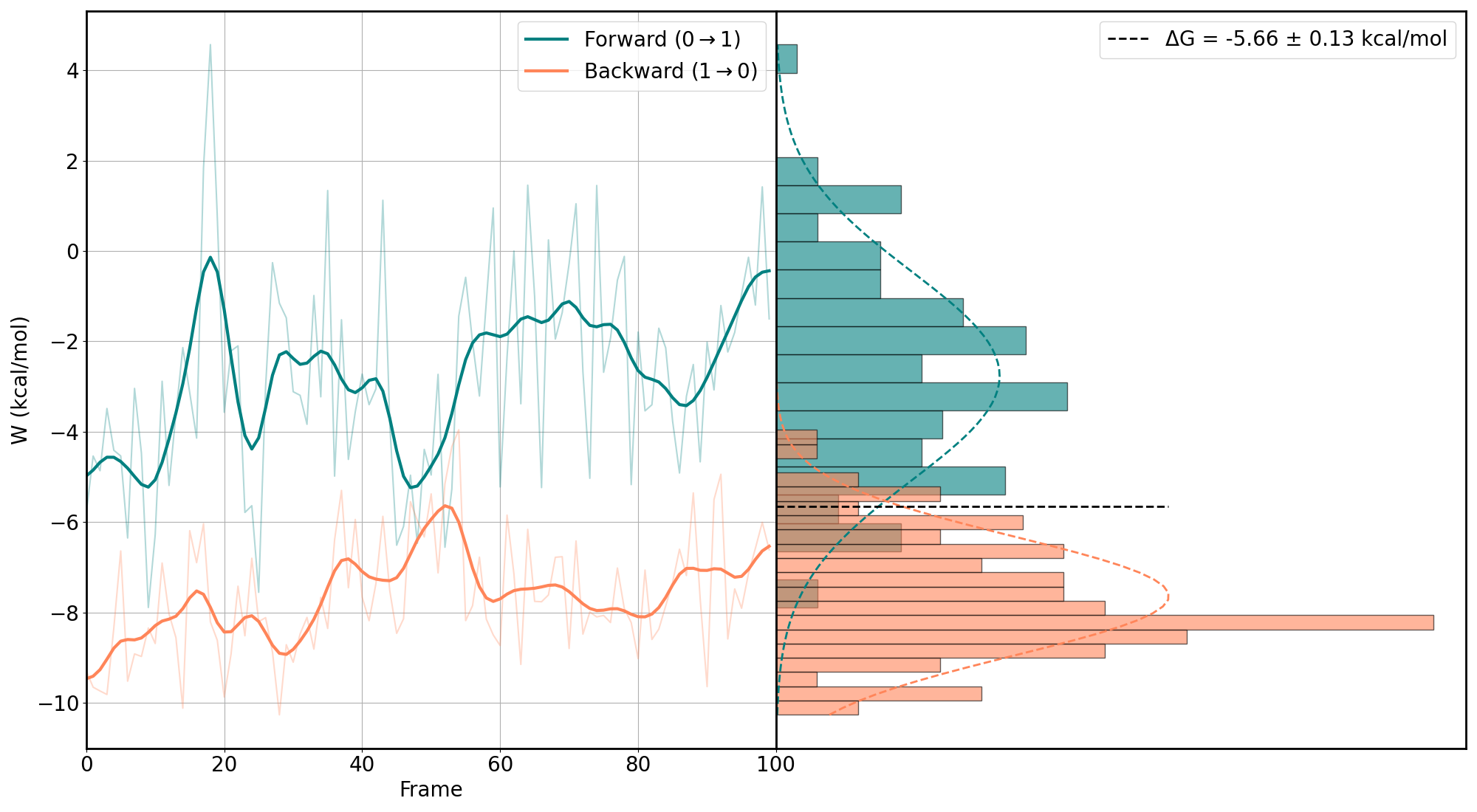
You want as much overlap as possible. More overlap means less error in the predicted free energy. Usually, the water alchemical transformation has good overlap, and the difficulties come with the membrane-embedded protein (MEP) or, sometimes, at the membrane.

You can easily modify the colors of the plot using the color_f and color_r in the input.yaml.

In order to obtain the final value for every \(\Delta G\), a weighted mean is performed so that if one value seems off (for example, because there is nearly no overlap), its weight is low.

Inside every edge, you will find a summary of the results in the image named results.png:

This contains, in a graphical way, the results of the results_summary.csv. You can tune the number of decimals (precision, recommended no more than 3) and use:

nemat img

To redo all the images without redoing the analysis.

9.4 Validation.

Use nemat val to print the validation test for every edge after the analysis has been performed. NEMAT will check the overlap of the forward and backwards transitions. If the overlap is \(\ge 0.2\), then it is considered a good overlap. Use this validation to check if the results make sense or not. Loads of non-overlapping results might lead to incorrect results. Therefore, if that’s the case, try increasing the number of transitions in the analysis or making them longer (not more than 1 ns since it’s non-equilibrium FEP).

This is not imperative. You may have a good system with low overlap. However, it is useful to know this metric.